For those of you just joining this blog, I roughly divided my protein folding project into two phases:

1. Discover how to extract from the PDB a vast set of local structure constraints that a special purpose constraint solving algorithm would use to fold proteins.
2. Develop the special purpose constraint solving algorithm.

Lucky for you, phase 1 is now complete! And as for myself, now that the effects of the celebration (clinking of Belgian beer goblets, emotional speech, etc.) have somewhat subsided, I mark the occasion in this post with a report on the local structure library that will be used in phase 2.

So as not to lose sight of the intended use of the folding algorithm, suppose we are given a primary sequence, say VEITELSER… , as input. To generate the constraints we first partition this sequence into overlapping subsequences of length four: VEIT, EITE, ITEL, TELS, etc. . For each of these we search for perfect matches in the PDB, extracting just that piece of the structure associated with the four-residue sequence.

I’ve carried out such searches for 100 four-residue sequences that were generated by a Markov chain based on residue digram frequencies. The first element of my chain happens to be VEIT. My settings of the PDB advanced search interface had the following criteria/parameters:

     macromolecule type: protein, no nucleic acid
     number of chains in biological assembly: 1
     sequence motif: VEIT
     x-ray resolution: 2 Å
     retrieve: representatives at 30% sequence identity

The last criterion, set at the lowest value provided by the interface, means that two proteins that happened to have the sequence VEIT in common are probably completely unrelated, and that any similarity in structure surrounding this group of residues is due to chemistry rather than ancestry, and therefore transferable as a candidate structure for the protein we are trying to fold. Performing this search on today’s date yields 28 hits — from 4P48 (“The structure of a chicken anti-cardiac Troponin I scFv”) to 1UTE (“Pig purple acid phosphatase complexed with phosphate”).

Extracting the local structures from the 28 PDB files is almost trivial. Each local structure comprises 4+1 atom positions, and 4+1 identifiers. The first four identifiers are just “VEIT”, and the α-carbon coordinates of these residues in the PDB file are the first four atom positions. The extra identifier is either “O”, when VEIT makes contact with a solvent oxygen atom, or a residue name when the contact is with a residue elsewhere in the protein. In the solvent case, the oxygen atom coordinates are the position of the extra atom, while in the residue contact case it is the coordinates of the contacting residue’s α-carbon.

For most hits there is just a single instance of the four-sequence motif (VEIT) in the protein. But associated with this single group of residues there can be, and usually are, multiple local structures as defined by the extra atom. For example, the first hit for VEIT, in the protein 4P48, yields five structures. In one of these the contact is with solvent, and in the others it is with residues C, L, T and T (in a different position). The only part of the local structure extraction process that requires any computation is identifying the extra atoms. In the solvent-contact case I require that the oxygen has distance below 4.5 Å from a side-chain atom in two of the residues; in the residue-contact case “oxygen” is replaced by “some atom in the contacting residue side-chain” and the cutoff is set at 5 Å. Finally, the residues in the motif making contact are required to be at positions 13, 24, 14 or 23. Here, for example, is the local structure record for the C contact:

V E I T C
40.125 13.719 8.71
37.928 14.317 5.657
37.717 17.818 4.177
35.781 20.008 1.738
44.898 15.387 5.989

There are 164 local structures for VEIT in the PDB (possibly more at lower x-ray resolution). The C contact is actually quite rare: only one instance. On the other hand, there are 18 V contacts and therefore a better chance of seeing the same one in different molecules. Here are two of them:

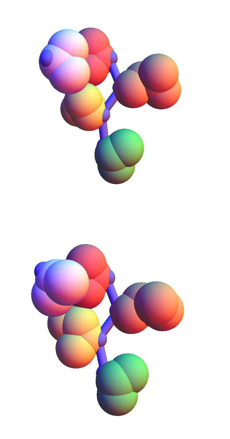
Backbones are colored purple, the side-chain atoms by residue: red (V), orange (E), yellow (I), green (T). Contacting residues (and solvent O) are always colored white. The valine (V) in these structures makes contact with the two non-polar residues in VEIT. The most popular contact for VEIT appears to be with solvent (52 instances). Here are two of them, with similar structure, selected from different proteins:

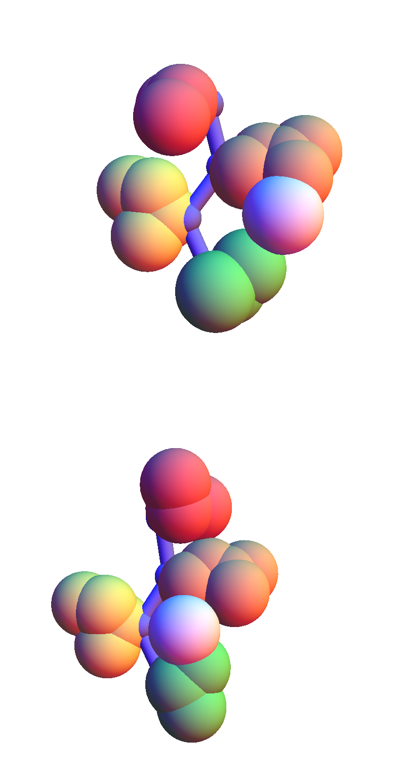
The contacting residues are now the polar pair, E and T.

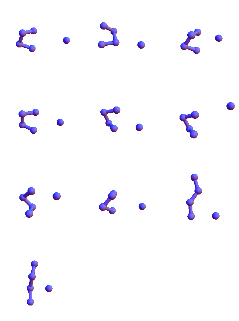
To get a better sense of the scope of these structures, here are all the solvent-contact structures for VEIT when these have been reduced to a maximal set of representatives, no two of which have RMSD (root-mean-square-deviation) less than 1 Å:

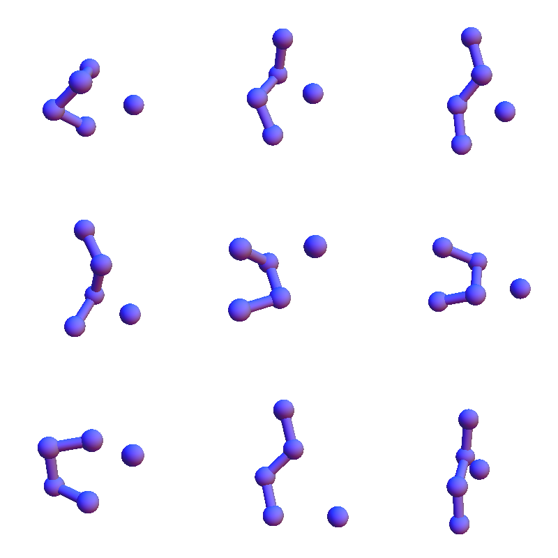
I show only the 4+1 α-carbon/solvent-oxygen atoms because the constraint satisfaction algorithm in my future will only work with these. These structures are in many respects different from the solvent-contact structures for the purely non-polar sequence FAAL that appeared later in my Markov chain:

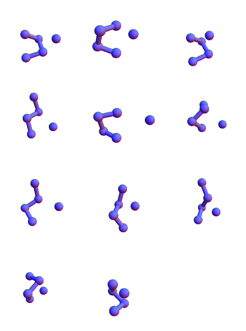
Unlike VEIT, non-solvent contacts are very popular with FAAL. A different way of rendering the diversity of, say, the L contacts, is to make a graph where two structures are joined by an edge when their RMSD is less than 1 Å:

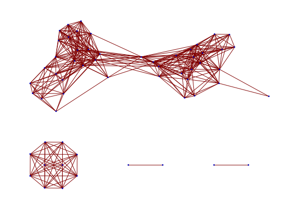
Mathematica’s embedding of the graph indicates there are three major structure types. On the other hand, if we choose to reduce all the PDB structures to a set of representatives, again at 1 Å resolution, we get the following set:

If I had to choose one result from the last week that best captures my optimism on the status of phase 1 it is the following plot of the “matching probability”:

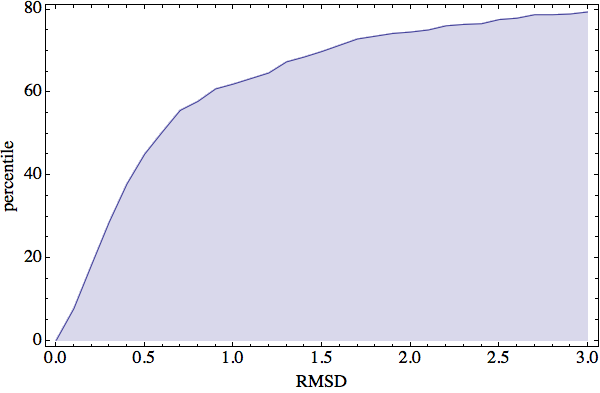
This plot answers the following question: What are the chances that the local geometry at some four-residue motif of protein X, whose structure is currently not known, is within some RMSD of a local structure for the same motif in a protein whose structure we can look up in the PDB? For example, at 1 Å RMSD we see that this probability is over 60%. This translates to a probability of better than 60% that we can find the correct constraint for any four-residue motif on the protein we are trying to fold. Of course, to understand why there is no actual penalty for “choosing the wrong constraint” one needs to have some idea of how my constraint satisfaction algorithm works. But that’s too much for this post. I’ll simply say that the selection of constraints, or deciding when to ignore them, is neither fixed at the outset nor something that needs to be sampled by exhaustion. 

The 60% probability of having available the correct match (at 1 Å resolution) is fantastic, considering the fact that each residue belongs to four motifs and therefore participates in 2.4 constraints on average. However, be sure to tune in next week when I go over all the ways that even with this success, phase 2 might still fail!