Not surprisingly, this first week of research was almost entirely carried out in the comfortable computing environment provided by a particular software package. This is not the only mode in which I work. I learned my craft in the days of scribbling page after page of equations on paper, and on some projects that is still how I spend my time. But not this week.

The nature of the work at this stage is very much driven by data. Over the years I've become proficient with the software package Mathematica (and a regular contributor to the Stephen Wolfram Private Island Fund). Without ever leaving this application, I can read .pdb files from the Protein Data Bank, render samples of the local structures I am interested in, generate my own data abstractions, and even write prototypes of the C programs that will eventually fold proteins. Whenever you see a plot or drawing in this research blog, it was probably generated in Mathematica.

Sunday

I used the advanced search feature of PDB to download .pdb files to get a first sampling of structures, restricting the search to pure protein (no nucleic acids, ligands) and structures with a single chain in their asymmetric unit. The only quantitative constraints imposed were the chain length, 100-500, and the X-ray resolution, 0.5-1.5 Å. At the bottom of the search interface I chose not to retrieve just one representative of sequence-similar structures because the mutation sensitivity of structures will be important. My laptop now has 303 new .pdb files!

Using Mathematica I found that some of my structures had pieces of chain with unknown (X) residues. Eliminating these, I ended up with 235 single-chain proteins, all with high quality structures.

The first significant action was deciding on the residue length of my local structures. Three is too short, because a backbone of just two bonds doesn't even encode the twist of the alpha-helix. Four might be enough, but I ended up picking five because an alpha-helix segment of that length is long enough for the residues at the two ends to be in proximity (and have an interaction):

In addition to the positions of five consecutive α-carbon atoms, each local structure also includes the α-carbon elsewhere on the chain that is closest to the central atom of the five. When the distance to this sixth atom is small enough it is designated as the "backbone contact"; otherwise, the sixth atom is eliminated from the local structure with the interpretation that the central atom makes contact with solvent.

After extracting all 39668 local structures from my 235 proteins, I made the following histogram of the distances (in Å) between the middle and contact atoms:

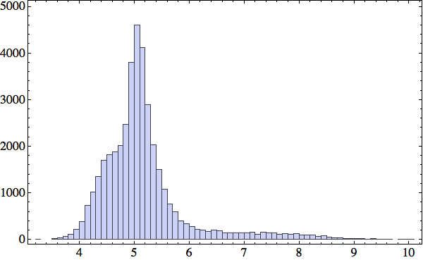
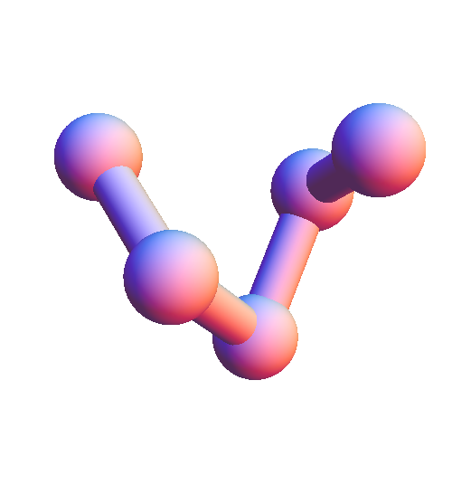
There is an interesting shoulder in the distribution around R=4.5 Å, suggesting that this might be the distance to use for selecting between backbone and solvent contacts. The exact value of this somewhat arbitrary criterion will not compromise the method of constraints I plan to use to fold proteins. Each five-residue subsequence will predict either a backbone contact or solvent contact; in the latter case the constraint satisfaction algorithm will simply make sure that a sphere of radius R centered on the central atom does not contain any backbone atoms (other than the four that are directly adjacent to the central atom along the backbone). Not wishing to miss any actual contacts, I chose R=4.8 Å. I now have 28352 local structures that have solvent contact and 11316  with backbone contact. This example shows how I represent (in Mathematica) one of the latter:

{
 {{"A", "A", "A", "M", "N"}, "G"},
 {
  {{8.097, 2.843, 5.583},
   {6.033, 5.103, 3.361},
   {8.6, 7.92, 3.485},
   {11.072, 5.392, 2.052},
   {9.006, 4.774, -1.075}},
  {7.569, 11.727, 4.122}
 }
}

Here we have three alanine (A), a methionine (M), and an asparagine (N) sequentially on the backbone, and the third A makes a backbone contact with glycine (G). The final three coordinates are those of the G. The contact distance in this structure is 4.00 Å; for comparison, the mean distance between adjacent α-carbons on the backbone is about 3.8 Å.

Monday

It's time to start assessing the completeness of the local structure library. The library would be judged "complete" if, given any string of five consecutive residues of a protein of unknown structure (so not yet in our local structure library), we could find several instances of that residue string in our library. Not only that, but the structures associated with those library items might have more than one form and we better have several instances of each of those forms. We should be uneasy if "several" had to be replaced by "a few", since then our sampling of local structures would be running the risk of having completely missed some cases.

The information in the current PDB is certainly insufficient to meet this high standard of completeness. If all 20^5 residue subsequences occur in natural proteins, and each adopts only a single local structure (surely an underestimate), then the library would need to hold tens of millions of items before we would be satisfied that our sampling is complete. My current library of 39668 local structures falls seriously short of that.

But I'm not all that concerned about these numbers. This local structure library differs in a significant way from a standard library. Think of the 5-residue subsequence as the "call number", and the structure (α-carbon positions) and contact residue as the "content". The central hypothesis of this project is that the content, at the resolution that matters to the folding problem, is relatively small in overall size: 21 contact residues (including solvent) times a few hundred geometries. Our library thus has very many copies of few books, and each copy has a different call number.

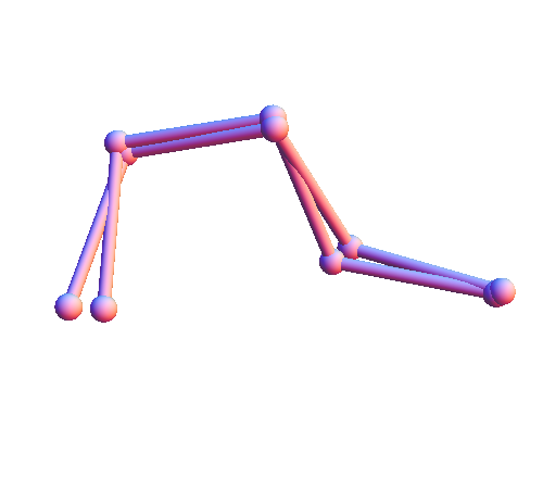
To make this all more quantitative I decided to discretize my local structures. First I wrote a Mathematica function, rbProj[x_,y_], that performs "rigid body projection". The argument x is a "target" set of points and y is a "template" having the same number of points. The output of rbProj is a rigid body motion applied to y that brings it as close as possible to x. For any pair of structures x and y (sets of points) I compute their distance as the norm of their difference after allowing for a suitable rigid body motion: dist[x_,y_]:=Norm[x-rbProj[x,y]]. Here are two local structures from my library (of the solvent contact type), where one has been translated and rotated to minimize the mean squared distance between corresponding atoms:

Riding home on the bus I reviewed the strategy I have all along been planning to use for retrieving items from the structure library. This "default" strategy is to map residue subsequences into a Euclidean space and then retrieve items close to a subsequence query by the Euclidean distance. A physics colloquium last fall by Nigel Goldenfeld inspired me to consider maps based on Carl Woese's polar requirement. But on this bus ride (20 minutes) I was determined to come up with a strategy that didn't rely on a biologically motivated distance.

Here's the scheme I dreamed up. Represent each 5-residue "call number" in my library as a binary sequence (22 bits) and concatenate it with its "content" (structure and contact residue), likewise represented as a binary sequence (about 15-bits, after discretization). To predict the content of queried call numbers we first construct a giant, conjunctive-normal-form Boolean formula. Clauses are generated at random and are tested for consistency against all the 37-bit items in the library (binary 0 and 1 correspond to truth values). Inconsistent clauses are rejected and consistent ones are added to the formula. Clauses with many literals have a good chance of being accepted, but are poor at generalizing, and vice versa. Retrieving content with the formula is done by setting the 22 call-number bits and exhausting on the 15 content bits that make the formula true.

I will keep this strategy in reserve. The feature I like most is that it naturally returns content as a set.

Tuesday

I started out following up on my plan of discretizing structure. To keep the computations manageable, I looked at just the 28352 solvent contact structures and selected a random 2000-item subset of those. The histogram of the structure distances between all pairs presented a surprise:

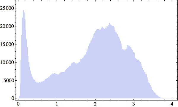
What's up with that peak near zero? A simple explanation (as to why there are unusually many structures all very near each other) popped out when I mapped the 2000 structures to a discrete set. I constructed my discrete set by using Mathematica's maximal independent set function to select a maximal subset of structures such that the distance between any two is greater than a given bound (this defines adjacency on the graph). Setting the bound at 0.5 Å (to include the peak in my distance histogram), I ended up with 200 structure representatives. Finally, I partitioned the 2000 structures into 200 sets according to which representative each is closest to.

Not surprisingly, one of the partitions was much larger than any of the others, and accounted for fully one third of all the structures in my sample! When I rendered one of these structures it was as if the clouds had parted and Linus Pauling's face grinned down at me: a 5-residue piece of alpha-helix. Of all local backbone conformations, the alpha-helix motif is unique in that its structure is defined entirely by hydrogen bonding among peptide atoms and therefore independent of the residues ("call number").

Wednesday

I woke up remembering a dream. In the dream I was in a room with strangers, participating in a group game whose rules I barely understood. As luck would have it, I was the first to be asked one of the puzzle questions: "What word is furthest both from itself and its opposite?" I remember asking the judge if by "opposite" she meant "antonym". When she nodded yes, I thought for a few seconds and blurted out "a synonym of the word". With relief I saw the judge smile: I had passed this round. But in the harsh light of wakefulness I'm not so sure. Worse yet, if this is a protein folding hint it leaves me in the dark.

Thursday

I've suddenly grown fond of a distance measure between residues based on mutations of the genetic code. Surely something like this must have been proposed before; it may even be related to the polar requirement. Consider the residue alanine. There are four RNA codons for this residue: GCT, GCC, GCA, GCG. Protein evolution, you would think, should lead to the situation where an isolated point mutation in the genetic code does not mess up the fold. Applying one point mutation to the four alanine codons we get 28 codons altogether, and these code for eight residues: A, D, E, G, P, S, T, V. This seems like a lot, but  remember that the idea is that at most one such residue-mutation will occur in each 5-residue call number. Averaged over all residues there are 8.5 mutations per residue, or about 42 mutations for each 5-residue subsequence that should be able to have the same structure. I plan to use this factor of 42 to boost the reach of the PDB.

Below is a graph I prepared showing all the residue mutations (edge connected pairs):

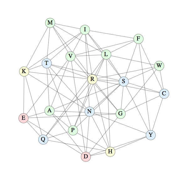
The color scheme is blue for polar residues, green for non-polar, yellow for basic and red for acidic. It's interesting that these properties only partially correlate with the connectivity of the graph.