In the early morning hours of October 16, humming within a computer in a basement office on the campus of Cornell University, the program litemotif 4.0 folded its first protein.

I’m setting that line in italics all by itself to give you the opportunity to hear it again, say in the resonant baritone of a Morgan Freeman or David Attenborough. The celebrations at Schoellkopf Field, while well timed, were actually part of the special Homecoming events in this sesquicentennial year of the University. Thank you Cornell. Your fireworks conveniently filled an awkward void.

The celebratory practices of individual researchers and small teams, unlike the throngs at mission control or Higgs particle announcements, are poorly documented. While we roll our eyes at scenes like the high-fiving Will and Prof. Lambeau in Good Will Hunting, it’s clear that those breakthrough moments cannot go unobserved. My friends in graduate school had a theory, in the case of Prof. Stanley Mandelstam, that major breakthroughs were celebrated by the purchase of a new sport jacket: “Look, he’s wearing N=4 SUSY-Yang-Mills finiteness.”

So what did I do? Simple: I prepared the graphics for this blog.

But before I display the amazing results, let’s go over exactly what happened on October 16. Before leaving Cornell for the day, I started six runs of litemotif 4.0 on the residue sequence for the protein 2P5K on a computer called “retriever”. There is nothing special about 2P5K — just one of a set of 32 small proteins I’ve been using to debug the program.

2P5K has the 63-residue sequence,

NKGQRHIKIREIITSNEIETQDELVDMLKQDGYKVTQATVSRDIKELHLVKVPTNNGSYKYSL.

The first step is to prepare the input file of litemotifs. For this I am indebted to Alex Alemi and Hyung Joo Park, who wrote a python program that extracts all applicable litemotifs from the PDB for any target sequence. Starting with NKGQ, for example, it retrieves all instances of α-carbon backbone coordinates for that 4-sequence and one other “contact” atom, either another backbone carbon or a solvent oxygen. A total of 24 litemotifs were found for NKGQ, 29% of which were solvent contacts. Similarly, for the next 4-sequence, KGQR, 101 litemotifs were retrieved, etc. On average, there were 278 litemotifs for each 4-sequence. When the algorithm folds 2P5K it is forced to pick just one litemotif coordinate-set for each 4-sequence.

We took care to remove from the input file all litemotifs native to 2P5K. The blueprints for folding this protein were thus obtained from diverse, functionally unrelated proteins. In a real folding exercise we would of course not have the native fold and native litemotifs available. The litemotif method distinguishes itself from other PDB-enabled folding schemes in the smallness of the motifs. Litemotifs are chemical entities and can therefore claim to cut across biological boundaries. I do not use the prefix “lite” lightly.

The folding algorithm, tasked with finding backbone and solvent atom positions that match all the chosen litemotifs, itself takes a number of parameters. The most important of these were the subject of the previous two posts. For the ADMM iteration I chose the “discrepancy accumulation” parameter value α=0.02. And for the minimum number of backbone contacts I chose 47; the algorithm determines which 47 of the 4-sequences will serve in this role.

The first evidence that 2P5K had folded came from the time series of the ADMM constraint discrepancy in run number 5:

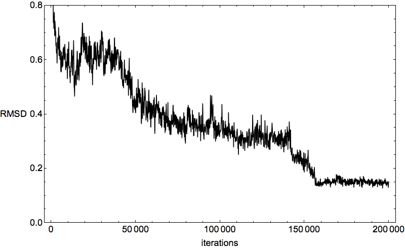
You’ve seen this kind of plot before, when I was debugging the program. Then I used just the native litemotifs, and the algorithm was held to the high standard of converging to zero discrepancy. Now, with the native litemotifs removed, convergence to zero discrepancy is plausibly imperfect. Consider it an amazing fact that it gets as small as it does!

Further evidence that 2P5K had settled down into something special after 150,000 iterations (5 hours) is the movie of the backbone and solvent atoms:

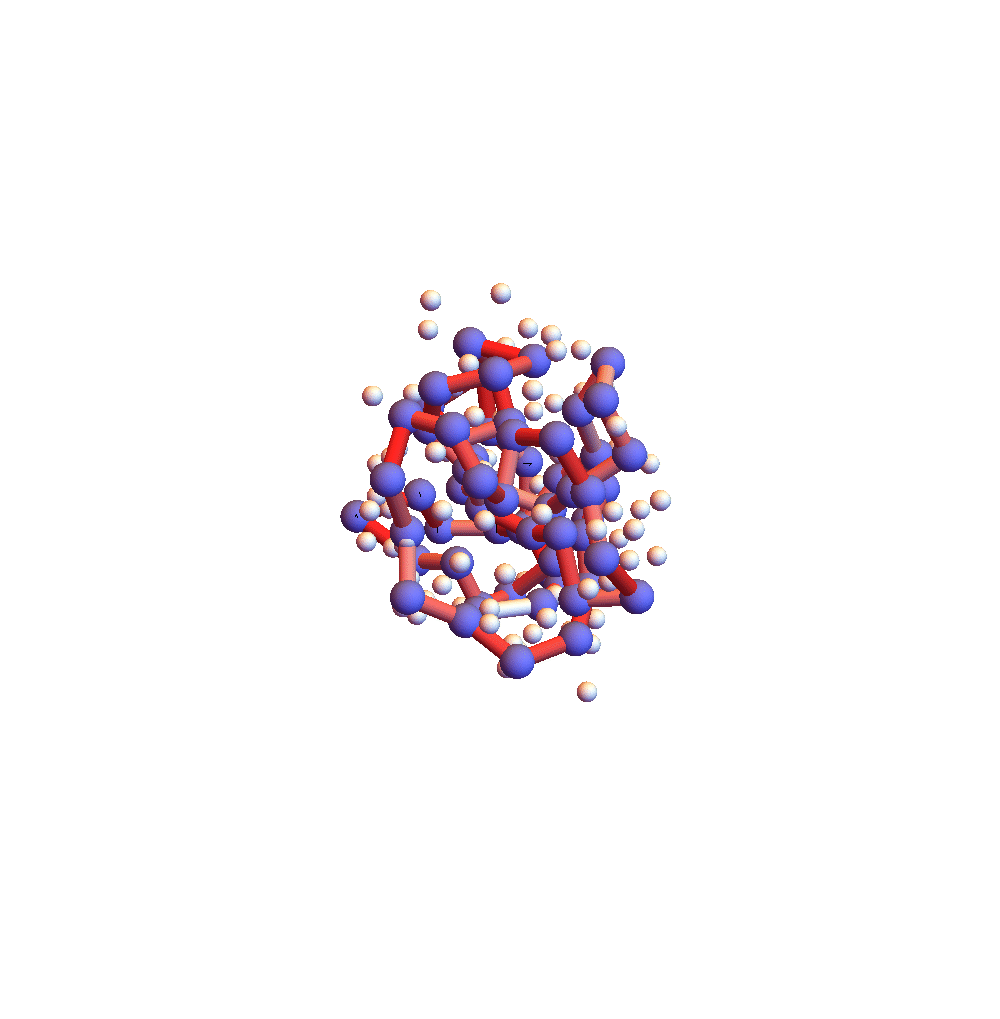
Notice that near the end of the movie (after iteration 150,000) the backbone appears to rotate as a rigid body. Because the centroid is fixed at the origin, rigid rotation is the only mode of motion that remains when all the backbone constraints are (approximately) satisfied. Movie frames are separated by 4000 iterations, and the redness of the backbone corresponds to the root-mean-square deviation of the current choice of litemotif (pink: RMSD = 1Å, red: RMSD > 2Å). 2P5K starts out blushing, for failing to select the correct litemotifs, and finishes in a cool shade of grey. A few points on the backbone remain red because I’ve set 5 as the number of litemotif constraints that can be ignored (for lack of samples in the PDB).

The final proof that the correct fold was found is the backbone rendering below:

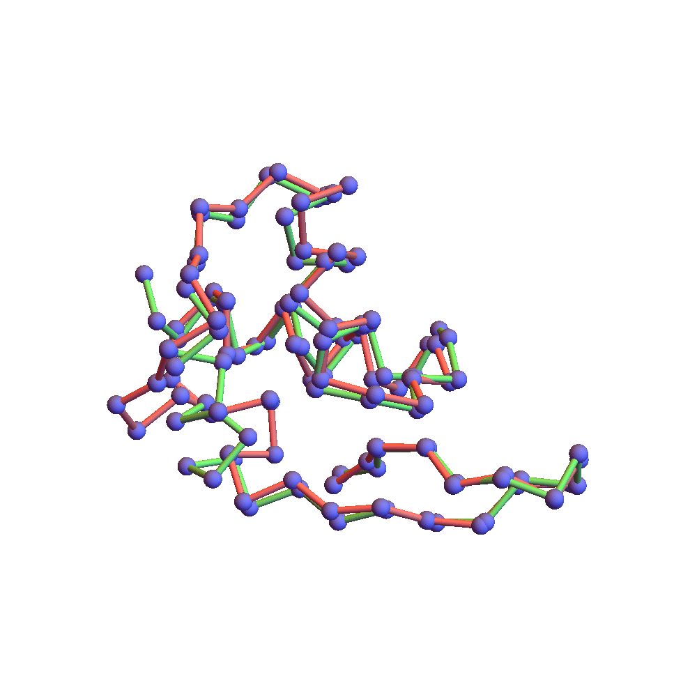
This compares the native backbone, in green, with the backbone found by the algorithm, in red, after one is aligned with the other by a rotation. Because the algorithm’s backbone is still slightly fluctuating due to the finite discrepancy, I used a few iterations of alternating projections (ADMM with α = 0) to get a unique solution for the comparison. The RMSD of the two folds, red and green, is 2.78Å. This is as good as anyone hopes for in the protein folding business. The remaining disagreement can usually be fixed up by handing the fold to a molecular dynamics package such as CHARMM or AMBER. Some of the disagreement is large, albeit localized on the backbone. The wrong bend at one of the ends might be fixed by using a special litemotif library for terminal 4-sequences.

Well there you have it. No chest-bumping with my laptop. The event is reported and I can get back to being a scientist.