I would like to think that the combined exhalations of relief, delivered from my followers worldwide on the reboot of the blog, could amount to a wind of sorts. And then I remind myself that this is not that kind of blog, but an experiment in real-time research documentation. In fact, I cannot rule out at this time that my readership comprises a single high school student in Estonia. In any case, welcome back and let me explain why Vabaduse tuul ei puhu!

The first half of my 2015 sabbatical is in Palo Alto, the site of Stanford University. Propelled by the fierce wind of freedom (from shoveling snow and interminable committee work), Liz and I drove cross-country to this mythical institution of higher learning and vanishingly low precipitation. But before I get to my actual reason for being here, a remark about the Stanford motto: The wind of freedom blows.

Stanford administration and trustees please note: your motto is severely compromised by the lens of present-day, student-age vernacular. And preserving the historical record is a poor defense in your case, as TWOFB has already undergone two transformations. Originating with Ulrich von Hutten’s third Invective at the Diet of Worms, videtis illam spirare libertatis auram, it then arrived in the German language as Die Luft der Freiheit weht. I therefore offer the following solution: simply substitute “stirs” for “blows”. The original meaning would be upheld, perhaps even amplified. After all, freedom is a subtle force, the very opposite of a category-5 hurricane.

I am here not because of Stanford, but to experience first-hand the workings of the Linac Coherent Light Source (LCLS), located at the Stanford Linear Accelerator Center (SLAC) just west of the campus. My project here is to see what can be done to mitigate “parasitic scattering”, perhaps the single-most serious obstacle to imaging individual (non-crystallized) biological particles.

Well then, where do things stand with the protein folding project? I’m sorry to report that the original litemotif concept is not tenable: even after fine tuning, protein 1ULR casts an ugly dissonance on my grand scheme.

Let me review as briefly as possible the original litemotif approach to protein folding and then move on to its failings.

Protein structure was reduced to the geometry of the sequence of CA (“alpha” carbon) atoms in the poly-peptide backbone of the molecule. The structure of the backbone would be constrained by the possible structures of short subsequences, and how these make contacts with other points on the backbone, or with solvent atoms. For short enough subsequences — I eventually chose four — the hope was that the information capacity of the “residue-to-geometry channel” was sufficient for all the local constraints to uniquely determine the geometry of the entire sequence (of course up to overall translation and rotation). The codewords of this channel, called “litemotifs”, were extracted from the PDB and given to a  geometrical constraint satisfaction algorithm.

In the first half-dozen protein folding experiments the results were spectacular. The algorithm had no trouble retrieving the correct litemotif to apply at each point of the backbone, even when there were hundreds of options (from the litemotif library) in each case. In those experiments I was careful to eliminate from the constraint library all native litemotifs, that is, constraints derived from the target fold itself. But those successes crumbled when it turned out that the litemotifs given to the folding algorithm were non-native in name only. The PDB often contains multiple versions of the same structure, usually differing on scales much smaller than what we care about in the folding problem. It still is remarkable, though, that the folding algorithm was able to correctly find all those needles-in-haystacks. But that does not diminish the embarrassment of giving the algorithm information that would not be available when folding a completely new protein!

The 4+1 litemotif scheme (4 backbone + 1 contact) unraveled with 1ULR. Even after making the detection of contacts more chemically informed, and allowing for wildcards when residues of the 4-subsequence made no chemical contacts, the algorithm never managed to find the native fold when care was taken to purge the litemotif library of near-identical versions. Below, for comparison, are the native backbone and the backbone of one of many folds that the algorithm did manage to find:

Your can trust your instincts here on selecting the failed fold: it is the ugly one.

What 1ULR brought home to me is the fact that there are powerful constraints that are poorly captured in the 4+1 scheme. In 1ULR these constraints are on display in a beautiful way, through its well defined secondary structures of alpha-helices and beta-sheets. I will kick-off this first posting of the new year by sketching a new litemotif scheme that at least is efficient for the representation of secondary structure.

The new scheme has both 3+1 and 3+3 litemotifs. Of the latter there are two kinds, and one of these corresponds to secondary structure. In this posting I only have time to describe the secondary-structure motifs. These are a huge departure from the old 4+1 scheme just by the fact that they are residue-blind: we do not need to know the six residues of the 3+3 group to know whether they apply.

Between every pair of consecutive CA atoms in the backbone there are four other peptide atoms in a planar quadrilateral:

One diagonal of the quadrilateral links consecutive CA’s while the atoms at the ends of the other diagonal, O and H, are responsible for hydrogen bonding. Three consecutive CA, or one half of the 3+3,  span two quadrilaterals and provide four possible hydrogen bonding atoms. In the 3+3 “secondary-structure litemotif” one hydrogen bonding atom in each quadrilateral of one “3”  makes a bond with counterparts in the other “3”. I define a hydrogen bond by the criterion that the distance, always between one O and one H, is less than about 2.5 Å. If you didn’t follow all of that just now, here’s one possible hydrogen bonding scheme in a 3+3 (CA = gray, O = red, H = white):

Those two consecutive hydrogen bonds between a pair of 3’s are strong constraints! I found 721 such instances in a set of 32 small proteins and the geometries of the six CA atoms are all within 1Å of one of the 18 shown here:

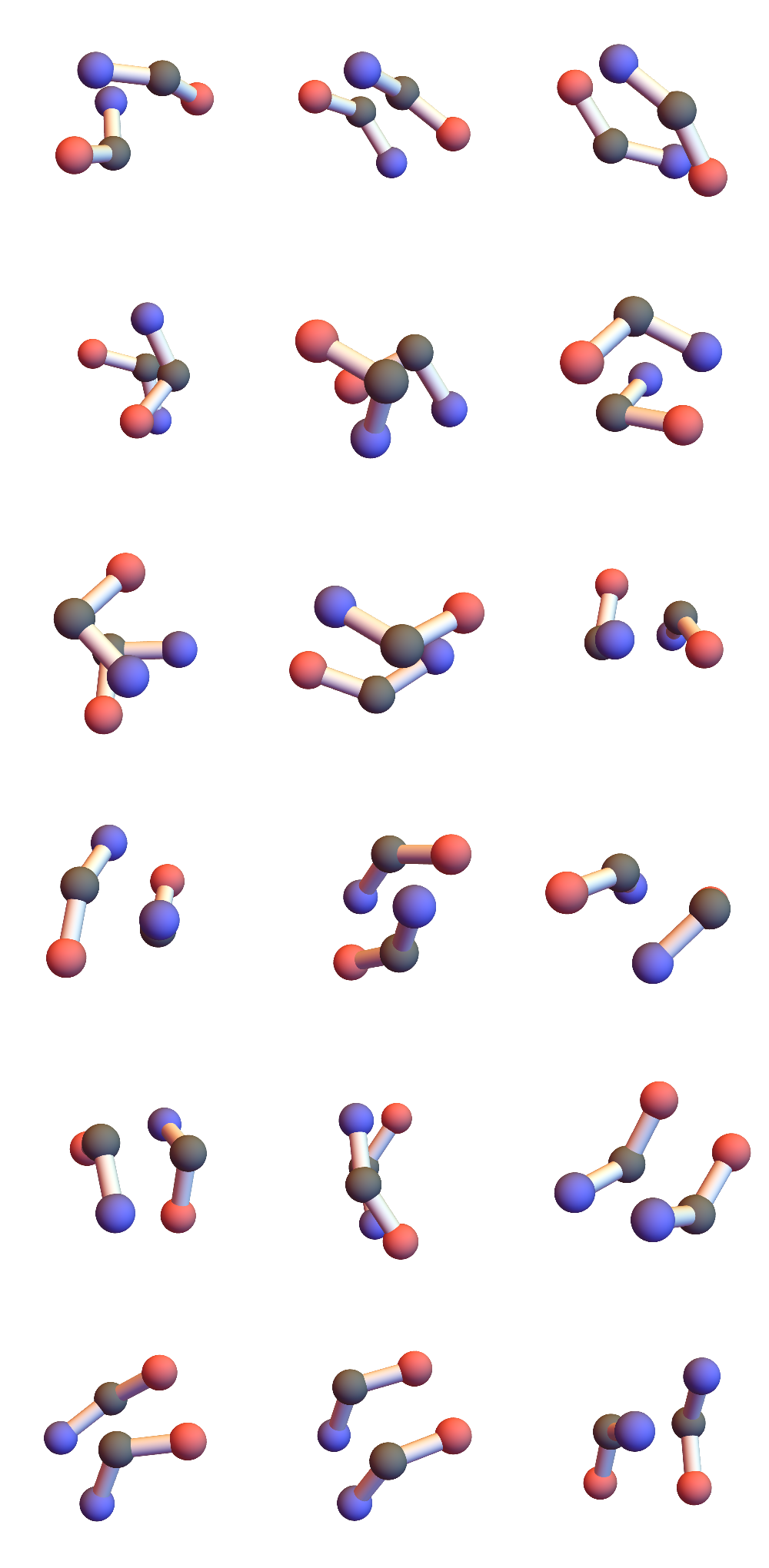
I’ve colored the CA atoms to convey the directionality of the chain. Red means the terminal peptide atom associated with that CA is O, blue when that atom is N. In alpha-helices and parallel beta-sheets the red and blue ends match; antiparallel beta-sheets correspond to unmatched-ends.

Most of 1ULR’s backbone is constrained by secondary-structure 3+3 pairs. Here I’ve rendered them with a red strut that joins the middle CA in each pair:

The beauty of those two helices (top) and that sheet (bottom) was completely missed by the old litemotifs! An 87-residue protein, 1ULR satisfies 42 of the new residue-blind 3+3 constraints. Not all proteins have this much secondary structure and not nearly as many of these constraints will be satisfied. Check out the blog next week to see what takes their place.